| Title Derive An Instantaneous Unit Hydrograph Using Clark's Method in GIS | |||||||||||||||||||||||||||||||||||||||||||||||||||||||||||||||||||||
|
Author Bryan Zhou American River College, Geography 350: Data Acquisition in GIS; Spring 2013 Contact Information: bryanlzhou@gmail.com | |||||||||||||||||||||||||||||||||||||||||||||||||||||||||||||||||||||
|
Abstract The unit hydrograph is a critical component in understanding hydrology. The unit hydrograph represents the relationship between runoff and watershed. The unit hydrograph can be estimated for basin lacking stream data using GIS and Clark (1945) method. The method requires three parameters: Time of basin concentration, Time-area map, and storage attenuation coefficient. The storage attenuation coefficient is used for routing the translate hydrograph. | |||||||||||||||||||||||||||||||||||||||||||||||||||||||||||||||||||||
|
Introduction The unit hydrograph is an important component in studying the relationship between watershed and runoff from precipitation. The hydrograph is function of rate of discharge over time in cubic feet per second (cfs). The unit hydrograph represents one unit of rainfall distributed uniformly for the entire basin. The graph of a unit hydrograph is derived from a stream gauged or storm data, but for a non-gauged basin, a synthetic unit hydrograph (instantaneous unit hydrograph) can be derived using several methods (Usul and Yilmaz). Clark (1945) is one such method and it is compatiable with Geographic Information System (GIS). The aim of this project is to derive an instantaneous unit hydrograph for the Mad River sub-watershed of Humboldt, CA using GIS. | |||||||||||||||||||||||||||||||||||||||||||||||||||||||||||||||||||||
|
Background Clark (1945) method is based on modeling the transportation of storm runoff from the stream channel to the basin outlet. The results are used to determine the isochrones (travel time of sub-basin). The isochrones and the storage coefficient are used to estimate a unit hydrograph. Clark’s method requires 3 important parameters, which are: :
Time of Basin Concentration The Soil Conservation Service (SCS) lag equation represents the time it takes for runoff to reach the basin outlet (Usul and Yilmaz). The National Operational Hydrologic Remote Sensing Center (NOHRSC) has provided the following equation for Tlag as: 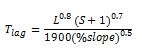
The weight raster (WGrid) represents the resistance to flow for each cell. In a given area, topography, vegetation, and land use are factors that influence the rate of flow. Water tends to move faster on an impervious surface or bare land, but moves slower in dense vegetation. Manning’s velocity (V) equation is used to create a Wgrid. The equation represents the velocity of surface runoff and it is converted into a raster layer known as VGrid. The modified version of the equation is provided below (Usul and Yilmaz). The nGrid represents manning’s roughness coefficient for each type of landuse class. The values for n can be obtained from literature. The RGrid represents the hydraulic radius (R), the ratio of the cross-sectional area of a channel to its wetted perimeter (the submerge portion of the channel). The RGrid is derived from Flow accumulation raster layer (FaGrid). A threshold value is applied to the FaGrid resulting in a stream network. The threshold value is based on the basin area and cell size of the DEM. Then, a R value is assigned to each group of flow accumulaiton value. A value of 0.001 is assigned to all non-stream network. The hydraulic radius values can be obtained from literature. The DEM is used to derive a slope raster (SGrid). The WGrid is created using the formula below (Usul and Yilmaz). Create Curve Number Map The Natural Resource Conservation Service’s runoff curve number (CN) is value representing the relationship of runoff and land use. The curve number is estimated from the combined soil and land use map along with the soil type, hydrologic soil group, and land categories. The hydrologic soil group (A, B, C, and D) represents the infiltration properties of soil type. Soil group A has the highest infiltration rate. Soil group B has moderate infiltration rate, while C and D being the lowest (Halley, White, and Watkins P.E.). Dr. Merwade devises a method for creating a CN raster that is suitable for hydrologic modeling and analysis. The requirement for creating a CN raster includes a DEM, soil data, 2006 land cover raster, and Hec-GeoHMS. The Hec-GeoHMS is hydrologic modeling software developed by the United States Army Corps of Engineers. Time-Area Map In a time area map, the basin is divided into areas of equal time intervals known as isochrones. Each isochrones represents the response time of runoff to the outlet for that area and it is represented as a histogram (NOHRSC). Three parameters are needed to create the isochrones: Tlag, FlGrid, and the maximum value from the FLGrid. The parameter is inserted into an equation provided below (Usul and Yilmaz). A translate hydrograph is created after computing the Area (% of basin area), the total volume of water, and discharge. The cell counts (Y-axis) and the cell size of the DEM are used to determine the Area. To determine the total volume of water, 1 unit of excess precipitation is applied to the whole basin (Area X 1 unit). The Area (%) and volume are converted into discharge. The final step is to route the translate hydrograph using the storage attenuation coefficient(Usul and Yilmaz). The basin or stream channel has the ability to store or prevent water from reaching the outlet. The value for R can only be estimated from a storm hydrograph using the following equation (NOHRSC). Alternative method in determining the storage coefficient is to use the natural logarithmic equation below. Qo and Qt represent the outflow and inflow rate at the time of the inflection point of the fallen limb (Noorbkhsh, Rahnama, and Montazeri, 2005). 
Then, the value for R is inserted into the following Constant equation below (NOHRSC). The final equation for linear reservoir routing is provided below:(Noorbkhsh, Rahnama, and Montazeri, 2005). IUHo = CIi + (1-C)IUHi-1 IUHi-1 represents the Y-axis of the translate hydrograph and Ii represents the time at end of the translate hydrograph (NOHRSC). | |||||||||||||||||||||||||||||||||||||||||||||||||||||||||||||||||||||
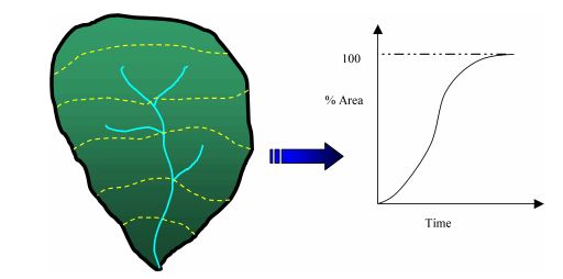
Figure 1: isochrone (NOHRSC) |
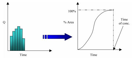
Figure 2: histogram (NOHRSC) | ||||||||||||||||||||||||||||||||||||||||||||||||||||||||||||||||||||
|
Methods The Mill Creek-Mad River watershed boundary (80 km2) was obtained from USGS National Hydrography Dataset. The soil shapefile and tabular data were obtained from the Soil Survey Geographic Database (SSURGO) and it can only be read with Access. The land cover raster (Figure 3) and the DEM (30 x 30 m) were obtained from the USGS. The DEM, soil, and land use maps were clipped to the watershed boundary. The Fill tool was used to remove errors (sinks) from the DEM. Then, the hydrology tools were used to create the flow direction and flow length raster. No Weight raster was created, because that part was optional. The soil raster was created using the Surface tool. 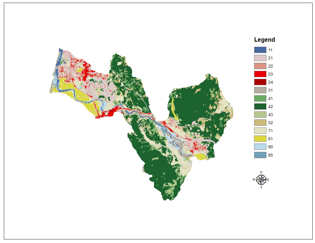
Figure 3: Land Cover Map The land cover map was converted into a polygon after determining the land use class with the aid of USGS land cover institute (LCI). The soil and land cover map were union together along with all the important elements (hydrologic soil group, land use class, PctA, PctB, PctC, and PctD fields). The fields contained the percentage of hydrologic soil group for each polygon within the area. All polygons with silvers were removed. A CN Look-up table (Figure 4) was created using values from TR-55 manual and Xu’s CN look up table. The table contained the curve numbers associated for each landuse class. After obtaining all the necessary parameters, Hec-GeoHMS for ArcGIS 9.2 was used to create a CN raster with a mean value of 79. 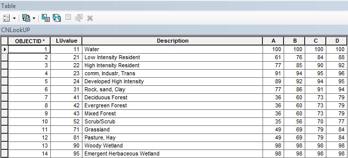 Figure 4: The CN Lookup Table The average slope for the basin was 14 percent. From the FlGrid, the maximum flow length for the basin was 19,228 m (63,068 ft.). The time of basin concentration was calculated to be 2.41 hours (no weight raster condition). The value for Tlag was used to create the time-area map (Figure 5). After truncating the time-area map, the Area between isochrones was calculated to be 28 km2, 41 km2, and 11 km2. Using the Mad River hydrograph from the California Nevada River Forecast Center, the storage coefficient was estimated as 1.31 hours. The final step involved using Dr.V.M.Ponce's online routing. The value from the area, duration of time (6 hrs), time interval (1 hr), and K were entering into the calculation module, which generated a table. 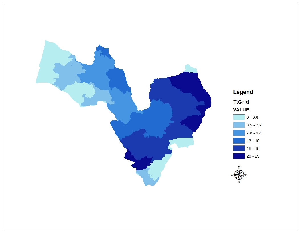
Figure 5: The Isochronal Map | |||||||||||||||||||||||||||||||||||||||||||||||||||||||||||||||||||||
|
Results The following table and graph shown below are the results from the online linear routing. The graph shows a higher and faster peak flow, because no weight raster was used for this unit hydrograph.
| |||||||||||||||||||||||||||||||||||||||||||||||||||||||||||||||||||||
|
|||||||||||||||||||||||||||||||||||||||||||||||||||||||||||||||||||||
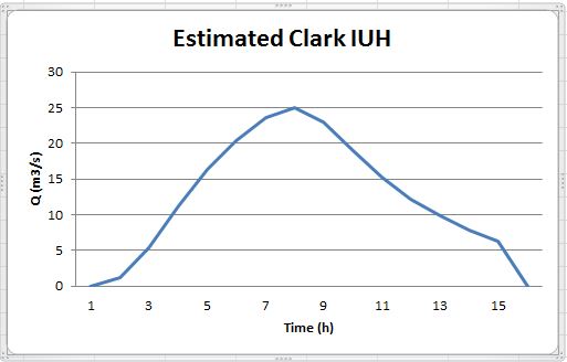
Estimated Clark IUH
| |||||||||||||||||||||||||||||||||||||||||||||||||||||||||||||||||||||
|
Analysis The USACE does not have a Hec-GeoHMS for ArcGIS 10.1, but older versions are available for download. The Hec-GeoHMS version for ArcGIS 9.2 was used for creating the CN raster, but the software failed to generate one due to a processing error. Another processing error occurred when attempting to create weight raster layer. The most difficult part of this project was estimating the storage coefficient constant. Due to insufficient research, the K value used for this project was only a crude estimated. Finding a histogram that resemble a translate hydrograph was also difficult. To save time, most of the remaining tasks was done on Dr. Ponce website. | |||||||||||||||||||||||||||||||||||||||||||||||||||||||||||||||||||||
|
Conclusions An unit hydrograph can be estimated for a basin lacking stream data using GIS and Clark (1945) method. Both the soil and land cover data do not accurately reflect the current conditions of the basin, because they are incomplete and outdated. Both of them are crucial in obtaining an accurate CN values. Another important thing for consideration is the use of a weight raster. The addition of a weight raster would of yield a more accurate unit hydrograph. The unit hydrograph would have a lower peak and a slower response time. The next step is to do more research on the storage coefficient and Manning’s principles. | |||||||||||||||||||||||||||||||||||||||||||||||||||||||||||||||||||||
|
References
Halley P.E., Marc C., S.O. White, and E.W. Watkins P.E."ArcView GIS Extension for Estimating Curve Numbers." ESRI Library:657.ESRI. Web. 2 April 2013. Merwade, Venkatesh, 2012. "Creating SCS Curve Number Grid using HEC-GeoHMS.School of Civil Engineering, Purdue University." Web. 5 April 2013. National Operational Hydrologic Remote Sensing Center, 2011: Unit Hydrograph (UHG) Technical Manual. NOAA. Web. 14 March 2013. Natural Resources Conservation Center, 1986: "Urban Hydrology for Small Watershed: TR55:165." PDF. United States Department of Agriculture. Web. 15 March 2013. Noorbakhsh, M.E., M.B Rahnama and S. Montazera,2005."Estimation of Instantaneous UnitHydrograph with Clark’s Method Using GIS Techniques." Journal of Applied Sciences 5(3): 455-458. JSTOR. Web. 13 March 2013. Ponce, V.M. 1999-2013, Prof. victor Miguel Ponce's website. onlinerouting07: Clark Unit Hydrograph. San Diego State University. Web. 24 April 2013. Usul, Nurunnisa and Musa Yilmaz. "Estimation of Instantaneous Unit Hydrograph with Clark’sTechnique in GIS." ESRI. ESRI Library:657.ESRI. Web. 13 March 2013. Xu, Allen L.,2006. "A New Curve Number Calculation Approach Using GIS Technology." Track: Water Resources. ESRI 26th Int’l User Conference. Web. 4 April 2013. | |||||||||||||||||||||||||||||||||||||||||||||||||||||||||||||||||||||